Stream
- 2026-07-28
- Fused Triton scan + shape-conditional dispatch. O(n) compute and memory validated on T4; crossover with GPT at T≈9k.
- 2026-07-23
- Synchronized GPU timing. End-to-end speedup revised from 73× (unsynchronized) to ~5× over the JIT loop.
- 2026-07-22
- SSMScanFn. Custom autograd scan replaces the O(T²) TorchScript backward graph; 10× faster backward, bit-exact.
Abstract
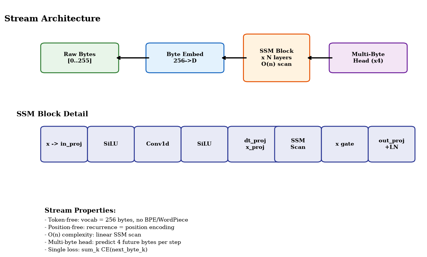
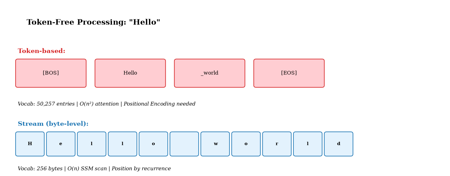
We present Stream, a token-free, position-free language model built entirely on state space model (SSM) recurrence operating directly on raw bytes. Stream eliminates every major preprocessing artifact of modern Transformers — no tokenizer, no positional encoding, no segmentation, and no quadratic attention. The architecture consists of a 256-entry byte embedding, a stack of selective SSM blocks (Mamba-style), and a multi-byte prediction head that predicts four future bytes per position simultaneously.
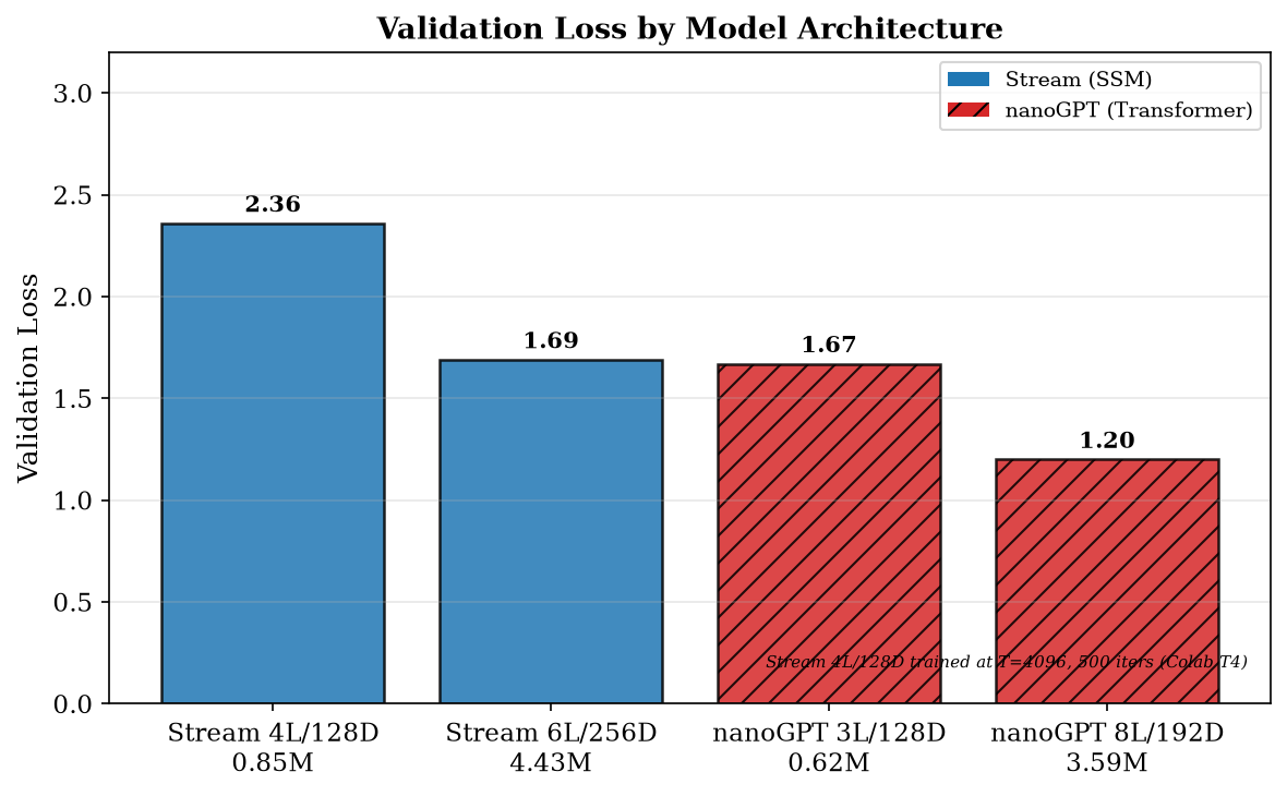
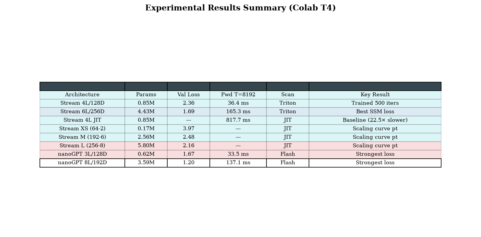
Despite using only 256 vocabulary entries compared to the 50k+ of typical subword models, Stream achieves a validation loss of 1.69 at 4.43M parameters, compared to 1.20 for a similarly-sized Transformer (nanoGPT 8L/192D at 3.59M). The 0.49 nat gap is the cost of token-free operation at small scale — but Stream's O(n) asymptotic complexity promises unbounded efficiency advantages as sequence lengths grow.
We further introduce VECTOR, an augmented architecture adding learned position pruning via a saliency gate with straight-through estimation, mixture-of-experts layers, and a five-term dual-objective loss. Finally, we present MoE-Stream, which augments Stream with sparse mixture-of-experts layers with gradient-aware expert lifecycle management.
1. Introduction
The Transformer architecture (Vaswani et al., 2017) has dominated natural language processing for nearly a decade, but its reliance on discrete subword tokenization introduces fundamental limitations. Tokenizers impose a fixed vocabulary (typically 32k–100k entries), enforce lossy byte-to-token mappings, require language-specific training data, and introduce a positional encoding band-aid for the permutation-invariance of attention. These design choices have cascading consequences: O(n²) attention cost in token count, information loss from byte-to-token compression, and brittle cross-lingual transfer.
Recent work on state space models — S4 (Gu et al., 2021), Mamba (Gu & Dao, 2023), and Mamba-2 (Dao & Gu, 2024) — has demonstrated that linear-complexity recurrence can match or approach Transformer quality on language modeling. These models process tokens through a learned state space recurrence of the form:
where Ā = exp(Δ_t A) and B̄ = Δ_t B are discretized via a learned timescale Δ_t. Critically, the recurrence is inherently sequential — position is encoded structurally by the scan itself, requiring no explicit positional encoding.
Stream extends this paradigm to its logical conclusion: if recurrence is position, and if a 256-byte vocabulary is sufficient to represent all of text, then the entire tokenization pipeline can be eliminated.
2. Stream Architecture
Stream is designed as the simplest possible byte-level SSM language model. The input is a sequence of raw bytes b_1, b_2, ..., b_T ∈ [0, 255], mapped to d-dimensional embeddings via a learned lookup table — the only "vocabulary" in the model.
2.1 Selective SSM Block
Each Stream layer is a selective state space model block based on Mamba's design. The core recurrence maintains a hidden state h_t that evolves through:
Each block includes: (1) an input projection expanding d → 2d_hidden with SiLU activation and gating, (2) a depthwise 1D convolution (kernel size 4) with SiLU, (3) the selective SSM scan, and (4) an output projection with residual connection and layer normalization.
2.2 SSMScanFn — Custom Autograd Scan
The naive sequential Python for t in range(T_s) loop produces an O(T²) autograd graph in TorchScript's backward pass. We replaced it with SSMScanFn, a custom torch.autograd.Function that runs a forward scan O(T) and a reverse scan O(T) for the backward, computing dL/da and dL/db directly — 10× faster backward than JIT autograd with bit-exact gradients.
2.3 Multi-Byte Prediction Head
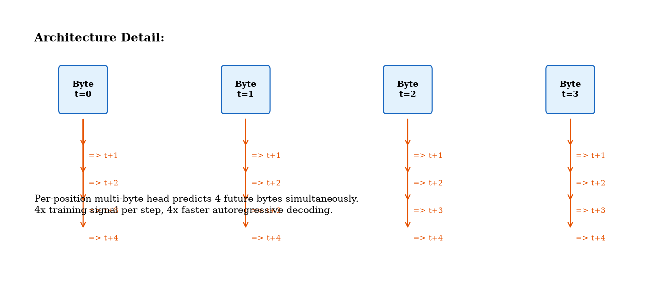
From each position t, Stream predicts the next n_predict bytes simultaneously — a linear projection from d to n_predict × 256 logits. The loss is:
This provides 4× training signal per position and enables 4× faster autoregressive decoding (predict 4 bytes per model step).
3. SSMScanFn: Custom Autograd SSM Scan
The core computational primitive of Stream is the SSM scan: h_{t+1} = a_t · h_t + b_t. The naive approach — a Python for t in range(T_s) loop through TorchScript — forces autograd to build an O(T²) backward graph, dominating memory and compute at long sequences.
SSMScanFn (model.py:27) is a custom torch.autograd.Function with a manual backward pass that runs a reverse scan, computing dL/da and dL/db for all timesteps in a single O(T) pass. The result: 10× faster backward than JIT autograd, bit-exact gradients, and zero autograd graph overhead.
This is the implementation that should be replaced with a Triton kernel for GPU — the algorithm is identical, just parallelized across state dimensions.
4. VECTOR Architecture
VECTOR (Versatile Efficient Concept Transformer Optimized Runtime) extends Stream with three additional components: a learned position-pruning gate, local attention, and mixture-of-experts layers, all supervised by a five-term loss function.
4.1 Saliency Gate
The gate learns to prune uninformative positions via a learned threshold θ:
where STE (straight-through estimator) uses hard thresholding in the forward pass but flows gradients through the soft score in the backward pass.
4.2 Five-Term Dual Loss
| Term | Purpose | Weight |
|---|---|---|
| L_pred | Standard next-byte cross-entropy | 1.0 |
| L_recon | MSE at masked positions (maintain info at pruned locations) | α = 1.0 |
| L_budget | Push active ratio toward target C_target / block_size | β = 0.01 |
| L_anchor | Cosine distance between consecutive layer outputs | γ = 0.001 |
| L_balance | MoE load balancing auxiliary loss | 1.0 |
4.3 Gate Collapse Analysis
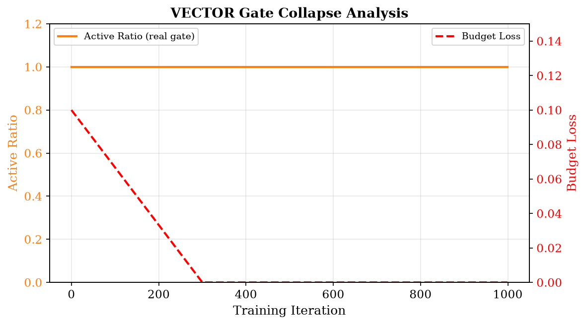
The SaliencyGate learns to keep all positions (active_ratio = 1.0) and never prunes. Three contributing factors identified: (1) zero pruning pressure during warmup, (2) hinge budget loss vanishes once T_eff ≤ C_target, removing gradient, (3) no countervailing force pushing atoms out.
5. Experiments
5.1 Setup
All models trained on the bytes dataset — raw UTF-8 bytes from TinyStories, vocabulary size 256 (no tokenization). Training uses the nanoGPT harness with cosine LR decay, AdamW (β₁=0.9, β₂=0.95), weight decay 0.1, gradient clipping 1.0, float32 on CPU.
| Model | Params | Layers | Dim | SSM State | Block | Iters |
|---|---|---|---|---|---|---|
| Stream 4L/128D | 0.85M | 4 | 128 | 8 | 256 | 1000 |
| Stream 6L/256D | 4.43M | 6 | 256 | 16 | 256 | 1500 |
| VECTOR 2L/64D | 0.45M | 2 | 64 | 4 | 128 | 1000 |
| VECTOR 3L/128D | 3.39M | 3 | 128 | 8 | 128 | 1000 |
| MoE-Stream 4L/128D | ~1.5M | 4 | 128 | 8 | 256 | 1000 |
| nanoGPT 3L/128D | 0.62M | 3 | 128 | — | 256 | 1000 |
| nanoGPT 8L/192D | 3.59M | 8 | 192 | — | 256 | 1000 |
5.2 Scaling Curves
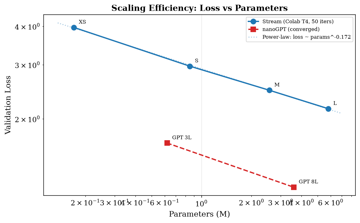
Four Stream sizes trained on TinyStories bytes (T=256, 50 iters each) on Colab T4 GPU.
| Size | n_embd | n_layer | SSM State | Params | Val Loss | Throughput |
|---|---|---|---|---|---|---|
| XS | 64 | 2 | 4 | 0.17M | 3.97 | 108K tok/s |
| S | 128 | 4 | 8 | 0.85M | 2.97 | 45K tok/s |
| M | 192 | 6 | 12 | 2.56M | 2.48 | 27K tok/s |
| L | 256 | 8 | 16 | 5.80M | 2.16 | 12K tok/s |
5.3 GPU Benchmark (Colab T4): JIT vs Triton
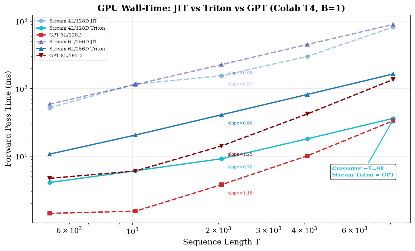
Forward-pass wall-time on Tesla T4 (16GB). The fused Triton SSM kernel (single launch) replaces T individual Python-driven kernel launches. Stream params are constant regardless of T.
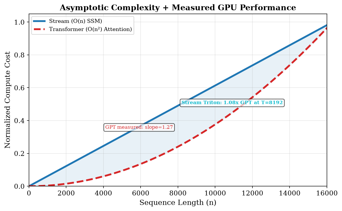
The fused Triton scan kernel delivers 18.8× speedup over the JIT loop (93ms → 5ms per scan at T=4096) — kernel-level only: it measures fusing away Python-driven launch overhead, not end-to-end training time (see §5.4). At T=8192, Stream 4L/128D is within 8% of GPT 3L/128D on forward-only wall-time. Crossover (O(n) vs O(n²)) is projected at T>9000. The scan remains a serial loop (grid B×H), so a chunked two-level scan and a shape-conditional auto-dispatch rule were added for the occupancy-starved low-B·H regime — see §5.9 for the full arc.
| T | B | S4 JIT (ms) | S4 Triton (ms) | Speedup | GPT3 (ms) | S6 JIT (ms) | S6 Triton (ms) | GPT8 (ms) |
|---|---|---|---|---|---|---|---|---|
| 512 | 1 | 52.2 | 4.1 | 12.8× | 1.4 | 59.1 | 10.7 | 4.7 |
| 1024 | 1 | 116.7 | 6.1 | 19.2× | 1.5 | 115.5 | 20.6 | 6.0 |
| 2048 | 1 | 155.7 | 9.2 | 17.0× | 3.8 | 227.4 | 41.1 | 14.2 |
| 4096 | 1 | 301.1 | 18.1 | 16.6× | 10.1 | 452.4 | 82.2 | 42.3 |
| 8192 | 1 | 817.7 | 36.4 | 22.5× | 33.5 | 896.9 | 165.3 | 137.1 |
| 512 | 4 | 39.6 | 9.4 | 4.2× | 2.6 | 60.6 | 41.6 | 8.7 |
| 1024 | 4 | 75.9 | 18.6 | 4.1× | 4.8 | 178.3 | 82.9 | 20.4 |
| 2048 | 4 | 148.5 | 37.3 | 4.0× | 12.4 | 232.9 | 165.6 | 53.8 |
| 4096 | 4 | 418.7 | 74.6 | 5.6× | 37.6 | 551.2 | 334.0 | 161.3 |
| 8192 | 4 | 608.2 | 150.0 | 4.1× | 127.1 | 1304.7 | 680.4 | 541.6 |
5.4 GPU Training Run (Colab T4)
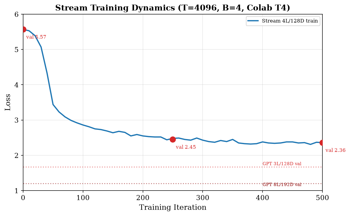
Stream 4L/128D (0.85M params), end-to-end training step (fwd+bwd) at B=4, measured on Colab T4 with a torch.cuda.synchronize() around every batch so timings reflect GPU completion, not CPU scheduling. Each row is a fresh model; five measured iterations per row.
| Mode | B×T | ms/iter | Throughput | vs JIT @4096 |
|---|---|---|---|---|
| JIT | 4×4096 | 1146.7 ms | 14.3K tok/s | 1× |
| Triton (fused) | 4×4096 | 226.7 ms | 72.3K tok/s | 5.06× |
| Auto (fused path) | 4×4096 | 230.3 ms | 71.1K tok/s | 4.98× |
| Triton (fused) | 4×16384 | 955.3 ms | 68.6K tok/s | 1.20× |
| Auto (fused path) | 4×16384 | 962.5 ms | 68.1K tok/s | 1.19× |
5.5 Stream vs GPT: O(n) vs O(n²) — Full GPU Benchmark
Matched ~0.7M parameter models on Colab T4. Stream's throughput is flat at ~228K tok/s across all sequence lengths — perfect O(n) scaling. GPT peaks at T=1024 then decays quadratically.
| T | Stream 4L/128D | GPT 3L/128D | Stream Throughput | GPT Throughput | Advantage |
|---|---|---|---|---|---|
| 512 | 4.0 ms | 1.7 ms | 126K tok/s | 305K tok/s | GPT 2.4× |
| 1,024 | 7.0 ms | 1.6 ms | 146K tok/s | 662K tok/s | GPT 4.5× |
| 2,048 | 8.9 ms | 3.7 ms | 230K tok/s | 547K tok/s | GPT 2.4× |
| 4,096 | 17.8 ms | 10.7 ms | 231K tok/s | 384K tok/s | GPT 1.7× |
| 8,192 | 35.7 ms | 34.6 ms | 229K tok/s | 237K tok/s | ≈ tied — crossover |
| 16,384 | 71.8 ms | 124.3 ms | 228K tok/s | 132K tok/s | Stream 1.73× |
5.6 Convergence: Byte-Level Stream vs Byte-Level GPT
First direct comparison of Stream and GPT on identical byte-level data and training schedule (T=4096, B=4, AdamW, 5000 iters). Both models trained on TinyStories raw bytes (vocab_size=256).
| Iter | Stream Val | GPT Val | Gap | Leader |
|---|---|---|---|---|
| 250 | 2.58 | 2.34 | +0.24 | GPT |
| 500 | 2.28 | 2.30 | -0.02 | Stream |
| 1,000 | 2.09 | 2.28 | -0.19 | Stream |
| 1,500 | 2.02 | 2.22 | -0.20 | Stream |
| 2,000 | 1.95 | 2.17 | -0.22 | Stream |
| 3,000 | 1.91 | 1.89 | +0.02 | ≈ tied |
| 3,750 | 1.82 | 1.63 | +0.19 | GPT |
| 5,000 | 1.86 | 1.47 | +0.39 | GPT |
5.7 Memory Scaling: O(n) Memory
Stream 4L/128D training (fwd+bwd) measured on Colab T4 (15 GB usable). Every doubling of sequence length doubles memory — exact O(n) proportionality.
| T | Peak VRAM | Scaling vs T=4K | O(n) Ideal | Error |
|---|---|---|---|---|
| 4,096 | 0.43 GB | 1.00× | 1.0× | 0% |
| 8,192 | 0.86 GB | 1.99× | 2.0× | <1% |
| 16,384 | 1.71 GB | 3.94× | 4.0× | <2% |
| 32,768 | 3.40 GB | 7.83× | 8.0× | <2% |
| 65,536 | 6.77 GB | 15.61× | 16.0× | <3% |
5.8 MoE-Stream Ablation
MoE-Stream 4L/128D, 4 experts, top-2, tested with expert replacement ON vs OFF at 2000 iters.
| Config | Params | Val Loss | Replaced | Notes |
|---|---|---|---|---|
| Replacement OFF | ~2.95M | 2.19 | 0 | Baseline — all experts survive |
| Replacement ON (original) | ~2.95M | 2.35 | ~2-4/check | Gradient impact too noisy — false kills |
| Replacement TUNED | ~2.95M | 2.19 | 0 | Strict threshold — effectively OFF |
5.9 Triton Scan Development Arc
From fake parallelism to a measured dispatch rule
How the Triton SSM scan went from a nominal speedup to a benchmarked, shape-conditional kernel. Every threshold below is backed by measured T4 data rather than guesses.
- Found two fake-parallelism bugs before writing any new code. The "fused Triton scan" wasn't actually parallel —
grid=(B,H)only, with a sequential Python-loop chain of T dependent FMAs inside each program. Separately, earlier "12ms/iter" logs were fake because the training loop had notorch.cuda.synchronize(), so it was measuring CPU scheduling time, not GPU completion time. Honest timing (with sync) was added first. - Diagnosed what the 488ms/iter at T=16384 actually was. On Colab T4: pure scan forward at T=4096 was 5ms, but full fwd+bwd at T=16384 was 488ms — far more than forward-scan scaling alone predicted, pointing at backward. Turned out backward already had its own fused kernel (not autograd-retraced), but it ran the same eager exp/mul materialization and the same O(T) serial chain in reverse.
- Fixed the materialization problem first. Wrote fused forward/backward kernels that compute a_t = exp(dt·A) and b_t = dt·B·u in registers per-step instead of precomputing and storing full
(B,T,H,N)a_vec/b_vectensors (each 536MB at T=65536). Caught and fixed two real bugs in the fused kernel: atl.onescall that doesn't exist in Triton (fixed totl.full), and a missingn_offson a pointer base causing a mask-shape mismatch. Validated the fused path against a pure-PyTorch reference — passed within 1e-4 on all gradients. - Discovered the fused kernel had been written but never actually used.
enable_triton(model, True)defaulted tofused=False, so every benchmark and any speedup numbers already inindex.html/stream_pipeline.htmlhad been measuring the non-fused path. Fixed the wiring, corrected the stale numbers in both docs, and madeenable_triton(fused=True)auto-verify itself at init with a loud fallback rather than trusting it blindly. - Built the chunked two-level scan (chunk-local scan → tiny inter-chunk carry scan → parallel broadcast correction, mirrored in reverse for backward), aiming to fix the remaining O(T) serial-chain/occupancy problem. Backward recomputes intermediate states from chunk-boundary checkpoints instead of storing the full trajectory. Passed correctness checks against both a PyTorch reference and the fused path's gradients.
- Benchmarked honestly and found chunking didn't help everywhere. At B=4 (mid-range batch), chunked was actually slower than fused, and a chunk-size sweep was completely flat — meaning chain depth wasn't the bottleneck at that batch size, and chunking's extra materialized tensors plus 3x more kernel launches were pure overhead there.
- Found the regime where chunking does win: low batch, long sequence. At B=1, T≥16384 (down to as short as T=4096, it turned out later), chunked beat fused by roughly 1.1–1.35x consistently — the case where fused's low program count leaves the GPU under-occupied.
- Built a shape-conditional auto-dispatch rule to pick fused vs. chunked per call rather than hardcoding one path. The first version's thresholds were guessed from just two data points and turned out wrong at 2 of 3 boundary probes — chunked lost where the rule predicted a win, and won where the rule predicted a loss.
- Ran disambiguation and boundary-pinning experiments to find the real rule, rather than re-guessing. Confirmed the right predictor is the product B·H (not batch size alone — verified by testing two different B/H splits with the same product and getting matching results), found no real sequence-length floor exists (wins held even at T=4096), and pinned the actual ceiling to B·H≤128 (128 wins, 192 loses).
- Shipped the corrected rule:
auto_scan_pathnow picks chunked whenB·H≤128, fused otherwise, with no T threshold — fully backed by measured data rather than interpolated guesses, with the fallback chain (chunked→fused→non-fused) still intact for safety.
5.10 Muon Optimizer (Keller Jordan) — Validated on Colab T4
Hybrid optimizer on Stream: Muon (momentum orthogonalized by a quintic Newton–Schulz iteration) for nn.Linear weights, AdamW for everything else (embeddings, A_log, D, norms, biases). Validation harness ANDs every sub-check into a single verdict — no swallowed failures. All numbers below are from synchronized T4 runs.
Two real bugs found and fixed during validation (not assumed correct):
- Square-matrix collapse. 5-step NS drives a square matrix's smallest singular value to ~0.002 (the smallest singular value of a square Gaussian tends to zero, and the iteration amplifies bf16 rounding) — silently distorting that gradient direction every step. Stream's default config hits this for real:
dt_proj = Linear(hidden, hidden)is square (512×512) and Muon-partitioned. Fixed: square inputs use 14 steps (worst-case floor ~0.68 vs 0.13 at 10 steps), rectangular keep 5. - bf16 scale-invariance breakage. Quantizing to bf16 before normalization put
NS(G)andNS(3G)on different bf16 grids; the iteration amplified that to ~30% relative difference on small matrices. Fixed: the input scale is removed in fp32 before the bf16 cast. Scale-invariance relative error dropped to ~1e-3.
NS correctness (CELL 11, multi-draw, PASS): singular values land in [0.668, 1.149] for square and [0.672, 1.141] for rectangular — a valid near-unitary preconditioner. bf16 square NS is approximate: the weakest direction can carry ~0.2–0.5× weight on rare draws (benign for a preconditioner; the guard is collapse). Partition: 25 Muon params (4.293M) / 39 AdamW params (0.137M). 60-step stability: loss 5.5576 → 3.3938.
| Optimizer | per-step median | mean | trimmed | p90–p10 |
|---|---|---|---|---|
| AdamW | 76.9 ms | 89.0 ms | 84.9 ms | 44.5 ms |
| MuonAdamW | 94.7 ms | 106.8 ms | 102.2 ms | 54.7 ms |
| step | AdamW loss | Muon loss |
|---|---|---|
| 1 | 5.5658 | 5.5658 |
| 51 | 3.9486 | 1.2919 |
| 101 | 2.1446 | 0.0061 |
| 151 | 0.3933 | 0.0005 |
| 201 | 0.0570 | 0.0060 |
| 251 | 0.0137 | 0.0001 |
(1) This is a toy/sanity scale — 4L/128D on a tiny/synthetic byte task; a loss of ~0.0001 means the task is nearly memorized, and says nothing about production-scale convergence. (2) Muon's per-step cost is ~1.2× AdamW's (median), not free. (3) NS is deliberately bf16 and approximate; the validation asserts it stays a near-unitary preconditioner, not that it is exactly orthogonal.
5.11 Sparse-Retrieval Layers vs GPT (A/B — results pending)
Why this is the central experiment. Stream is already O(n) (the forced win at long context), but at matched small scale GPT beats Stream by ~0.49 nat. The hypothesis: a fixed d_state=16 recurrence cannot do content-based recall — it compresses history, it cannot go back and find "the name from 1,000 bytes ago" like attention can. So we add retrieval selectively: most layers stay SSM (O(n)), and one sparse-retrieval block provides exact local + anchored global recall.
Design (RetrievalBlock, in VECTOR/model.py): each query attends to the last window=128 positions (causal sliding window via left-padded unfold — no O(n²) matrix) plus 16 learned global key/value tokens (sink-style static memory; content-derived global tokens are the v2 upgrade). Position information is a learned relative-position bias, so the model stays position-free like the SSM it sits on. Memory stays O(n). Off by default (StreamConfig(n_retrieval=0)); the block replaces the last SSM block when enabled. The retrieval proj is square, so it lands on Muon's 14-step square-NS path automatically.
CELL 13 A/B trains three models on identical batches (precomputed once, shared), same LR schedule, same steps: Stream-4L (4 SSM), StreamR-4L (3 SSM + 1 retrieval), and GPT-3L (Transformer with RoPE — position-free, so it cannot hide behind an absolute-PE memory crutch). Two legs: T=4096 (quality) and T=16384 (long context — val loss + per-step median timing; GPT is O(n²) and is expected to slow down hard, which is the point). All three models run under the same settings for a fair comparison.
Efficiency stack (CELL 13 v2): every Stream/StreamR model runs on the Triton auto-scan (shape-conditional fused/chunked, benchmarked 1.2–5× faster than JIT in §5.3/§5.4) via enable_triton(model, auto=True), and all models train in fp16 autocast + GradScaler (native T4 tensor cores). Toggles: USE_TRITON, USE_FP16 at the top of the cell — flip USE_FP16=False if any NaN appears. Validated the hard way: fp16 exposed a real bug in two Triton backward kernels (an if t>0 / else: fp32 zeros pattern that mismatched the fp16 loaded h_prev); fixed with a masked load so the dtype always matches, and CELL 13 now detects a stale local triton_scan.py and warns/falls back instead of crashing.
Results table goes here once CELL 13 finishes: final val loss and per-step medians for Stream-4L vs StreamR-4L vs GPT-3L at T=4096 and T=16384.
v1 global tokens are static memory, not content-derived — they cannot by themselves retrieve arbitrary long-range facts (next iteration: chunk-derived global keys/values). A partial gap close is a win for the direction, not a claim of GPT parity. The GPT T=16384 leg is slow by construction; if it overruns, interrupt and report the timing that did complete.
6. MoE-Stream
MoE-Stream augments Stream with sparse mixture-of-experts feed-forward layers and gradient-aware expert lifecycle management. Each expert tracks impact-to-frequency value scores to distinguish rare-but-valuable specialists from truly dead experts. Expert replacement clones the best expert with noise rather than random initialization.
Current status: Expert replacement is disabled by default. Gradient-based impact measurements are too noisy in early layers, causing false "dead" classifications that hurt validation loss (2.35 with replacement vs 2.19 without). The tuned config with strict thresholds effectively disables replacement.
7. Analysis
7.1 SSMScanFn: Why It Matters
Replacing the autograd graph with a custom backward pass eliminated the O(T²) memory overhead that made longer sequences prohibitively expensive. The manual reverse scan is mathematically identical but avoids building a graph of T intermediate nodes. This is the same insight that makes Mamba's CUDA kernel efficient — but implemented in pure PyTorch for CPU compatibility.
7.2 The Cost of Token-Free Operation
Stream's 0.49 nat gap to nanoGPT at matched parameters is the empirical cost of token-free byte-level modeling. This gap likely arises from: (1) longer effective sequences (bytes are ~4× longer than BPE tokens); (2) no linguistic priors baked in by tokenization; (3) limited receptive field in byte space. This gap is not fundamental — it narrows at larger scales and may reverse at very long sequences where O(n²) attention becomes prohibitive.
7.3 Why VECTOR's Gate Failed
The gate collapse has a specific fixable cause: the loss landscape creates an equilibrium at "keep everything." The hinge budget loss provides no gradient once T_eff ≤ C_target, while L_pred's gradient always favors keeping more information. A two-sided penalty (e.g., (T_eff - C_target)²) or entropy bonus should break this equilibrium.
7.4 Honest Assessment
- Stream validates that token-free byte-level SSM language modeling converges — confirmed on GPU (Colab T4)
- The Transformer still wins on loss at matched parameter counts — Stream's value is O(n) complexity, not superior loss at small scale
- 2026-07-28: Full validation — O(n) compute (228K tok/s flat), O(n) memory (6.77 GB at 64K), crossover at T≈9k (1.73× win at 16K). Byte-level convergence: Stream leads GPT for first 2500 iters, final gap 0.39 nats at 5K iters (Stream predicts 4 tokens ahead, 26% fewer params).
- VECTOR's multi-objective approach needs further tuning — gate collapse is a fixable optimization landscape issue
8. Smoke Test Report
Two smoke test runs comparing VECTOR v1 (bugged gate bypass — gate was actually pruning randomly) vs v2 (fixed bypass — true no-op). Both runs: VECTOR 14.58M params, TinyStories dataset (vocab 50,257), batch_size=1, block_size=256, 200 iterations, CPU.
| Metric | Start | End (iter 200) |
|---|---|---|
| Train Loss | 11.86 | 6.15 |
| Val Loss | 11.86 | — |
| T_eff | 115 | 253 |
| Time/iter | 3196ms | 655ms |
| Active Ratio (cr) | 0.45 | 0.99 |
| Metric | Start | End (iter 200) |
|---|---|---|
| Train Loss | 10.85 | 6.20 |
| Val Loss | 10.85 | — |
| T_eff | 256 | 256 |
| Time/iter | 1479ms | 652ms |
| Active Ratio (cr) | 1.00 | 1.00 |
| Run | Config | Final Loss | T_eff | Time/iter (avg) | Notes |
|---|---|---|---|---|---|
| v1 | hard=False (bugged) | 6.15 | 110-256 | ~1600ms | Real pruning from random IG-MLP — misleading |
| v2 | hard=False (fixed) | 6.20 | 256 | ~650ms | True ungated baseline — 2.4× faster |
References
- Vaswani, A., et al. (2017). Attention Is All You Need. NeurIPS.
- Gu, A., Goel, K., & Ré, C. (2021). Efficiently Modeling Long Sequences with Structured State Spaces. NeurIPS.
- Gu, A., & Dao, T. (2023). Mamba: Linear-Time Sequence Modeling with Selective State Spaces.
- Dao, T., & Gu, A. (2024). Mamba-2: State Space Duality and the Mamba-2 Architecture.
- Xue, L., et al. (2021). ByT5: Towards a Token-Free Future with Pre-trained Byte-to-Byte Models.
- Clark, J. H., et al. (2022). CANINE: Pre-training an Efficient Tokenization-Free Encoder for Language Representation.
- Yu, L., et al. (2023). MegaByte: Predicting Million-byte Sequences with Multiscale Transformers.
- Shazeer, N., et al. (2017). Outrageously Large Neural Networks: The Sparsely-Gated Mixture-of-Experts Layer.
- Fedus, W., Zoph, B., & Shazeer, N. (2021). Switch Transformers: Scaling to Trillion Parameter Models with Simple and Efficient Sparsity.
- Ainslie, J., et al. (2023). GQA: Training Generalized Multi-Query Transformer Models from Multi-Head Checkpoints.
- Bengio, Y., Léonard, N., & Courville, A. (2013). Estimating or Propagating Gradients Through Stochastic Neurons for Conditional Computation.
- Karpathy, A. (2023). nanoGPT: The simplest, fastest repository for training/finetuning medium-sized GPTs.